Landmarks (using Local Files)

Four scores are here computed to extract computation landmarks: structural, visual, cultural, pragmatic. The user has to provide at least an attribute shapefile containing the height attribute (the only mandatory field). See below for further instructions on the data sources.

The user can also provide, seaprately, information about cultural/historical landmarks (e.g. position of listed important buildings); see 3 - Cultural component

import sys
from pathlib import Path

repo_root = Path.cwd().resolve().parents[1]
sys.path.insert(0, str(repo_root))

import cityImage as ci
import matplotlib.pyplot as plt
import matplotlib.font_manager as fm

fm.fontManager.addfont("times.ttf")
plt.rcParams["font.family"] = "Times New Roman"

import pandas as pd, numpy as np, geopandas as gpd, osmnx as ox
from shapely.geometry import LineString
%matplotlib inline

import warnings
warnings.simplefilter(action="ignore")
pd.options.display.float_format = '{:20.2f}'.format
pd.options.mode.chained_assignment = None

import osmnx as ox
import cityImage as ci

Functions from the cityImage API used in this notebook

This notebook scores buildings as candidate landmarks, combining structural, visual, cultural and pragmatic salience into global and local imageability scores, starting from locally provided files.

• buildings_from_file — Load building footprints from a local file into the buildings schema.

• buildings_from_osm — Download building footprints from OpenStreetMap into the cityImage buildings schema.

• select_buildings_by_study_area — Restrict a buildings GeoDataFrame to those within the case-study area.

• plot_gdf — Plot a single GeoDataFrame with cityImage styling.

• structural_score — Compute the structural landmark component (distance from the network, 2D advance visibility, number of neighbours).

• compute_3d_sight_lines — Compute 3D sight lines between viewpoints and buildings for visibility scoring.

• visibility_score — Compute the visibility landmark component (facade area and, when available, 3D sight-line visibility).

• cultural_score — Compute the cultural landmark component from historical/cultural attributes.

• classify_land_use — Classify raw land-use values into cityImage land-use categories.

• pragmatic_score — Compute the pragmatic landmark component from land-use frequency.

• compute_global_scores — Combine the component scores into a global (city-wide) landmark score.

• compute_local_scores — Combine the component scores into a local (neighbourhood-relative) landmark score.

• plot_grid_gdf_columns — Plot several columns of one GeoDataFrame as a grid of maps.

For the full list of functions and their parameters, see the API reference.

Loading the Layers

Proive the input path where the building layer of the city/area of interest is stored. This file shouldn’t be exactly one’s case-study area but a larger area (e.g. not Boston’s city centre (case-study area), but the entire city of Boston).

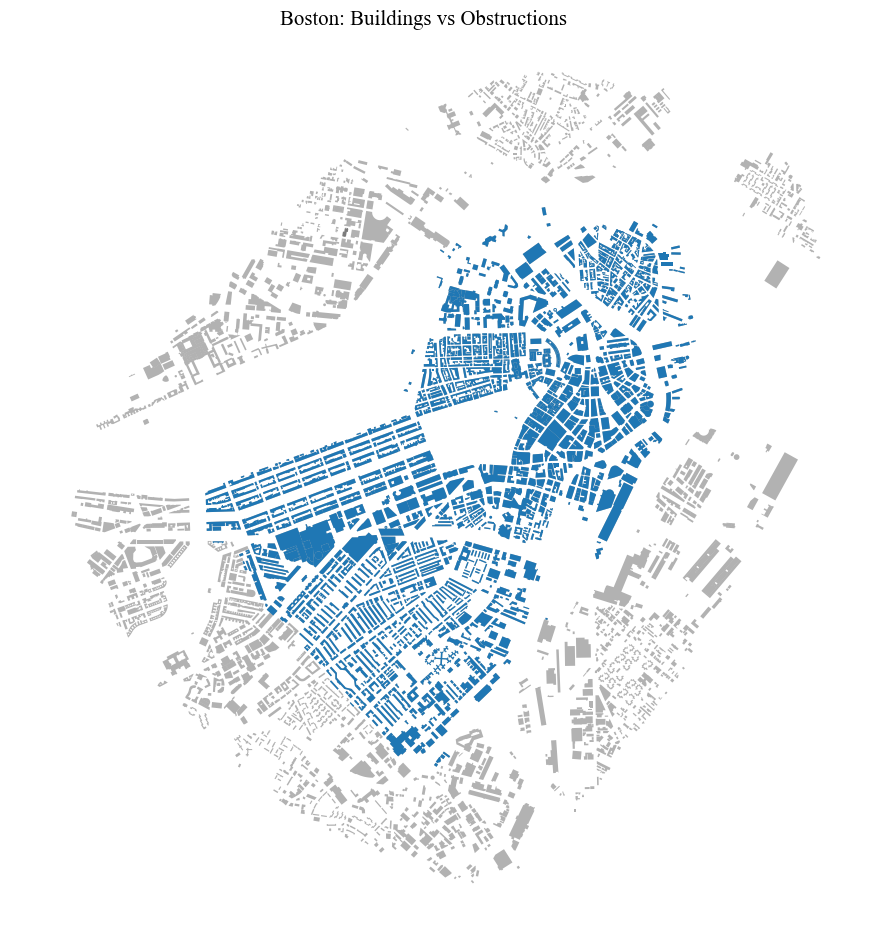
Landmarks are extracted from buildings that are within the chosen case-study area (buildings geodataframe). Other buildings around the case study area have to be included in the analysis in order to correctly compute the landmark measures, namely, to avoid that buildings located along the boundaries of the case-study area benefit from the fact that in the buildings geodataframe outer buildings are not included.

In other words, buildings is a subset of obstructions.

One can set option to:

• 1 - Load one’s buildings and obstructions gdfs from a local path. Choose when: Files are ready and contains the height, and a land_use fields.

• 2 - Get a large set of building from OSM (obstructions), extract the buildings, and attach information regarding height and land_use use from an existing file that it is in one’s possession (if this file is for example issued by an official data source and therefore more complete than OSM). This step makes sense only if one’s not comfortable with the shapes of the building footprints in their possession. Often these files contain footprints too precise and not fitting the purposes of this work. Instead, OSM provides already simplified footprints. Choose when: Having a shapefile with the height and land_use attributes but it is preferred to use the more simplified OSM geometries and attach the attributes to the OSM footprints.

• 3 - Load a buildings dataframe that would correspond to obstructions and obtain the buildings geodataframe by using a certain distance or a case-study area polygon (see below for details). Choose when: Having a shapefile containing buildings in a large area, including and outside one’s case study area; one is comfortable with the geometries and the height and land_use attributes are contained in such a file.

Buildings smaller than 200 square meters are kept out of the analysis, as well as buildings whose height is lower than 1mt (when the height field is filled).

In general, the obstructions geodataframe should include buildings located around 1000 m away from the boundary of the buildings gdf. This may vary, of course, on the basis of the analysis that one intends to conduct.

Ininitialising path, names, etc.

city_name = 'Boston'
epsg = 26986
crs = 'EPSG:'+str(epsg)
input_path = '../data/'+city_name+"/"
option = 3

# from local
case_study_area = gpd.read_file(input_path+city_name+'_studyArea.gpkg').to_crs(epsg=epsg).iloc[0].geometry

#specify the land use field's name in the file
height_field = 'height'
base_field = 'base'
land_use_field = 'landUse'

Defining the Layers

Option 1

Using already prepared buildings and obstructions datasets. One should be aware that buildings should be a perfect subset of obstructions. This means that all the buildings in buildings should be in obstructions, sharing the same attributes.

• The datasets should contain fields named base and height, representing the base height of the building (could be set to 0) and the height of the building.

• The buildingID should be already set correctly, that is, matching in the obstructionsand buildings GeoDataFrames.

if option == 1:
    buildings = gpd.read_file(input_path+city_name+'_buildings.shp').to_crs(epsg=epsg)
    obstructions = gpd.read_file(input_path+city_name+'_obstructions.shp').to_crs(epsg=epsg)
    buildings.index, obstructions.index = buildings.buildingID, obstructions.buildingID
    buildings.index.name, obstructions.index.name = None, None
    obstructions['land_uses_raw'] = obstructions[land_use_field]
    obstructions.drop(land_use_field, axis = 1, inplace = True)

Option 2

Download the obstructions from OpenStreetMap for a large metropolitan area that covers your case-study area, and (optionally) enrich them with height, base and land-use attributes taken from a local detailed-buildings file. The buildings GeoDataFrame is then obtained by restricting the obstructions to the actual case-study polygon.

This path uses buildings_from_osm, assign_building_heights_from_other_gdf, land_use_from_other_gdf and select_buildings_by_study_area.

# a large metropolitan area that fully covers your case-study area
place = ''  # e.g. "Boston, Massachusetts"
if option == 2:
    obstructions = ci.buildings_from_osm(place, download_method="OSMplace", crs=crs)

    # (optional) attach height/base and land-use attributes from a local detailed-buildings file
    attribute_file = gpd.read_file(input_path + city_name + '_detailedBuildings.gpkg').to_crs(epsg=epsg)
    obstructions = ci.assign_building_heights_from_other_gdf(
        obstructions, attribute_file, crs, base_field=base_field, height_field=height_field,
    )
    obstructions = ci.land_use_from_other_gdf(
        obstructions, attribute_file,
        new_land_use_column="land_uses_raw", other_land_use_column=land_use_field,
    )
    # NB: cityImage no longer ships a footprint-simplification helper; if your OSM
    # footprints are very detailed, simplify them with GeoPandas' geometry.simplify(...).

    # restrict the obstructions to the actual case-study area
    buildings = ci.select_buildings_by_study_area(
        obstructions, method="polygon", polygon=case_study_area,
    )

Option 3

If one doesn’t have a precise case-study area polygon to pass: Use the parameter distance_from_center to indicate till how far away from the center of the case-study area one wants to include buildings. When the user doesn’t provide the case-study area polygon nor the distance parameter, buildings and obstructions overlap; they have the same extent as the original input file.

height_field and base_field should indicate the maximum and the base elevations attributes of the buildings, in the original .shp file. When base_field is not provided, base is automatically set to 0. height_field is necessary to perform the landmark extraction. If such a feature is not at disposal, one should set height_field to None.

if option == 3:
    obstructions = ci.buildings_from_file(
        input_path+city_name+ '_obstructions.gpkg',
        crs,
        case_study_area=None,
        distance_from_center=None,
        height_field=height_field,
        base_field=base_field,
    )
    buildings = ci.select_buildings_by_study_area(
        obstructions,
        method="polygon",
        polygon=case_study_area,
    )

Optional readjustments

obstructions = obstructions[obstructions.geometry.within(buildings.geometry.unary_union.convex_hull.buffer(1000))]

obstructions

	height	base	area	landUse	geometry	buildingID
151	19.98	1.55	935.45	Residential Condo Unit	POLYGON ((237051.689 902972.866, 236990.897 90...	151
550	23.53	1.72	2466.09	Commercial Condo Unit	POLYGON ((237109.75 901488.558, 237000.835 901...	550
551	11.75	-1.29	526.52	Commercial	POLYGON ((237027.023 901476.82, 237001.853 901...	551
552	7.21	-0.38	292.29	Commercial Land	POLYGON ((237044.307 901416.818, 237004.172 90...	552
553	20.49	1.39	2620.96	Residential Condo Unit	POLYGON ((237142.368 901348.946, 237005.398 90...	553
...	...	...	...	...	...	...
6558	25.68	1.52	4086.12	Exempt	POLYGON ((232808.536 899562.8, 232828.761 8995...	6558
6559	16.56	1.95	1594.13	Exempt	POLYGON ((232822.026 899506.197, 232834.73 899...	6559
6571	16.93	1.41	2392.47	Commercial Land	POLYGON ((232887.683 899608.367, 232906.511 89...	6571
6572	27.70	1.17	3773.17	Commercial	POLYGON ((232814.013 899628.112, 232865.439 89...	6572
6573	10.37	0.95	743.39	Commercial	POLYGON ((232810.102 899634.308, 232858.034 89...	6573

2943 rows × 6 columns

obstructions['landUse'].unique()

array(['Residential Condo Unit', 'Commercial Condo Unit', 'Commercial',
       'Commercial Land', 'residential', 'Exempt', 'restaurant',
       'Apartments 7 Units above', None, 'Mixed Use Res/Comm',
       'Exempt 121A', 'commercial', 'Apartments 4-6 Units', 'Industrial',
       'Residential Three Family', 'industrial', 'apartments',
       'university', 'bicycle_parking', 'dormitory', 'education',
       'government', 'school', 'office', 'boathouse', 'hotel', 'parking',
       'retail', 'Condominium Master', 'house', 'service', 'construction',
       'college', 'terrace', 'Condominium Parking', 'shelter', 'church',
       'hospital', 'roof', 'emergency_service', 'garages', 'garage',
       'Residential Land'], dtype=object)

land_use_to_disregard = ['stockroom, warehouse', 'garage', 'stable', 'workshop','converter', ' pumping station', 'barracks', 'barn'
       'greenhouse', 'shed','greenhouse (botany)', 'bunker, shelter','heating plant', 'parking, garage',
               'electricity substation']
obstructions = obstructions[~((obstructions.landUse.isin(land_use_to_disregard)) & (obstructions.area < 200))]

obstructions = obstructions[~((obstructions.landUse.isnull()) & (obstructions.height.isnull()))]
height = obstructions[~obstructions.height.isnull()].height.quantile(0.25)
obstructions['height'] = obstructions['height'].where(obstructions['height'] > 0.0, height)
buildings = buildings[buildings.buildingID.isin(obstructions.buildingID)]

Visualisation. The cell below maps the result using the cityImage plotting helpers such as plot_gdf; see the Plotting section of the API reference for all styling options.

fig = ci.plot_gdf(buildings, scheme = None,  black_background = False, figsize = (10,10),
                  title = city_name+': Buildings vs Obstructions', base_map_gdf = obstructions, base_map_color = 'black',
                  base_map_alpha = 0.3)

Structural component

It considers:

• The area of the building.

• Its distance from the road.

• The number of adjacent buildings, within the given neighbours_radius, around it.

• A measure of 2d advance visibility, expanded till a maximum distance from the center of the building on the basis of the advance_vis_expansion_distance parameter.

# including outputs from previous notebooks
output_path = '../output/'+city_name

# reading the street network and passing it in the function to compute the structural score
edges = gpd.read_file(output_path+'_edges.gpkg')

# The 'buffer' parameter indicates distance within the algorithms look for neighbouring buildings
buildings = ci.structural_score(buildings, obstructions, edges, advance_vis_expansion_distance = 300,
                                neighbours_radius = 150)

Visual component

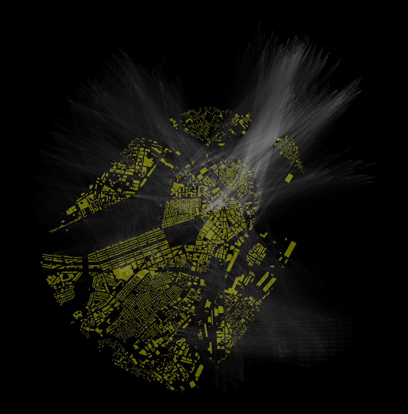
Sight Lines Construction

This is a computationally expensive step that may takes hours (in particular the intervisibility check that verifies whether the sigh lines are actually visible or not). One way to reduce it is to cluster nodes and therefore generate a lower number of sight lines. The function takes two parameters, besides the observer and the targets GeoDataFrames:

• distance_along: It regulates the interval along the exterior of each building for which a point is identified and used as a target point. If the exterior of the building is shorter than the parameter, at least one point is identified.

• distance_min_observer_target: The function only computes sight lines for nodes and buildings whose distance is higher than this parameter.

One can choose between two methods to compute the 3dvis score:

combined –> It computes a combined score that takes into account, per each building:

• The number of sight lines towards it.

• Their average length.

• The maximum lenght amongst them.

longest –> It just uses the longest sight line’s length as a score

buildings

	height	base	area	landUse	geometry	buildingID	road	2dvis	neigh
550	23.53	1.72	2466.09	Commercial Condo Unit	POLYGON ((237109.75 901488.558, 237000.835 901...	550	17.99	89352.63	20
551	11.75	-1.29	526.52	Commercial	POLYGON ((237027.023 901476.82, 237001.853 901...	551	17.84	38375.87	17
552	7.21	-0.38	292.29	Commercial Land	POLYGON ((237044.307 901416.818, 237004.172 90...	552	4.45	41101.49	16
553	20.49	1.39	2620.96	Residential Condo Unit	POLYGON ((237142.368 901348.946, 237005.398 90...	553	4.11	128536.86	15
554	12.17	1.15	793.82	Commercial	POLYGON ((237199.594 901363.43, 237197.299 901...	554	27.32	183974.08	7
...	...	...	...	...	...	...	...	...	...
6047	17.80	0.87	589.50	Residential Condo Unit	POLYGON ((236886.134 900440.682, 236853.291 90...	6047	11.50	77644.06	13
6048	7.47	1.32	351.20	Residential Condo Unit	POLYGON ((236937.198 900463.676, 236930.845 90...	6048	60.73	58691.63	8
6049	23.56	0.95	3609.91	None	POLYGON ((234702.34 900398.09, 234692.807 9004...	6049	6.48	19445.91	21
6050	71.55	4.72	4116.83	None	POLYGON ((236414.03 900412.087, 236313.318 900...	6050	4.47	8520.39	28
6051	33.24	0.77	5753.09	Commercial Condo Unit	POLYGON ((236873.645 900347.507, 236838.52 900...	6051	9.76	117504.70	13

1408 rows × 9 columns

# nodes = gpd.read_file(output_path+'_nodes.gpkg')
# sight_lines = ci.compute_3d_sight_lines(nodes, buildings, obstructions_buildings_gdf = obstructions, simplified_target_buildings = None, edges_gdf = edges,
#                                         city_name = "Boston",
#                                         distance_along = 300, min_observer_target_distance = 300, height_relative_to_ground = False, consolidate = False)

buildings = ci.visibility_score(buildings, sight_lines, method = 'longest')
buildings.head()

	height	base	area	landUse	geometry	buildingID	road	2dvis	neigh	fac	3dvis
0	23.53	1.72	2466.09	Commercial Condo Unit	POLYGON ((237109.75 901488.558, 237000.835 901...	550	17.99	89352.63	20	1282.19	0.38
1	11.75	1.00	526.52	Commercial	POLYGON ((237027.023 901476.82, 237001.853 901...	551	17.84	38375.87	17	325.96	0.03
2	7.21	1.00	292.29	Commercial Land	POLYGON ((237044.307 901416.818, 237004.172 90...	552	4.45	41101.49	16	171.90	0.38
3	20.49	1.39	2620.96	Residential Condo Unit	POLYGON ((237142.368 901348.946, 237005.398 90...	553	4.11	128536.86	15	1488.76	0.57
4	12.17	1.15	793.82	Commercial	POLYGON ((237199.594 901363.43, 237197.299 901...	554	27.32	183974.08	7	382.03	0.53

fig = ci.plot_gdf(sight_lines, alpha = 0.07, color = 'white', base_map_gdf = obstructions, base_map_color = 'yellow',
            geometry_size = 0.08, base_map_alpha = 0.4)

Cultural component

It measures the symbolic/cultural value of each building. This part is case-study specific, see other examples for generalizable methods

cultural_elements = gpd.read_file('../data/Boston/otherSources/'+city_name+'_historic_landmarks.gpkg').to_crs(epsg=epsg)
buildings = ci.cultural_score(buildings, cultural_elements)

Pragmatic component

Before computing the pragmatic score, the land_use_raw raw field is categorised into more granular categories. One can fill in the following categories to accomodate descriptors not accounted for. Essentially, the user needs to come up with land-use categorise and distribute the OSM’s ones (or from other sources) within these categories.

print(obstructions['landUse'].unique()) # to visualise the list of land uses to categorise

['Residential Condo Unit' 'Commercial Condo Unit' 'Commercial'
 'Commercial Land' 'residential' 'Exempt' 'restaurant'
 'Apartments 7 Units above' None 'Mixed Use Res/Comm' 'Exempt 121A'
 'commercial' 'Apartments 4-6 Units' 'Industrial'
 'Residential Three Family' 'industrial' 'apartments' 'university'
 'bicycle_parking' 'dormitory' 'education' 'government' 'school' 'office'
 'boathouse' 'hotel' 'parking' 'retail' 'Condominium Master' 'house'
 'service' 'construction' 'college' 'terrace' 'Condominium Parking'
 'shelter' 'church' 'hospital' 'roof' 'emergency_service' 'garages'
 'garage' 'Residential Land']

# introducing classifications and possible entries

adult_entertainment = ['brothel','casino', 'swingerclub', 'stripclub', 'nightclub', 'gambling']

agriculture = ['shed', 'silo', 'greenhouse', 'stable', 'agricultural and forestry',  'greenhouse (botany)',
               'building in the botanical garden']

attractions = ['attractions',   'attraction','aquarium', 'monument',  'gatehouse', 'terrace', 'tower', 'attraction and leisure',
               'information', 'viewpoint', 'tourist information center', 'recreation and amusement park',  'zoo',
               'exhibition hall, trade hall', 'boathouse', 'bath house, thermal baths', 'entertainment hall', 'sauna']

business_services = ['bank', 'service','offices', 'foundation', 'office', 'atm', 'bureau_de_change', 'post_office',
              'post_office;atm', 'coworking_space', 'conference_centre',  'trade and services', 'trade and services building',
                      'customs office', 'insurance', 'tax_office', 'post', 'administrative building',  'facility building',
                      'residential building with trade and services', 'data_center', 'tax office']

commercial = [ 'commercial',  'retail', 'pharmacy', 'commercial;educa', 'shop', 'supermarket', 'books', 'commercial services',
              'commercial land', 'car_wash', 'internet_cafe', 'driving_school', 'marketplace', 'fuel', 'car_sharing',
              'commercial and industry buidling',  'crematorium', 'commercial building', 'commercial and industry building',
              'commercial building to traffic facilities (general)', 'funeral parlor', 'gas station', 'car wash',
              'pumping station','boat_rental', 'boat_sharing',  'bicycle_rental', 'car_rental', 'dive_centre']

culture = ['club_house','gallery', 'arts_centre','cultural facility', 'cultural_centre', 'theatre', 'cinema', 'studio',
            'exhibition_centre', 'music_school', 'theater','castle', 'museum', 'culture']

eating_drinking = ['bbq', 'restaurant', 'fast_food', 'cafe', 'bar',  'pub', 'accommodation, eating and drinking',
                   'ice_cream', 'kitchen', 'food_court', 'cafe;restaurant', 'biergarten']

education_research = ['university', 'research', 'university building', 'education and research', 'research_institute',
                     'research_institu']

emergency_service = [ 'fire brigade','fire_station','police', 'emergency_service', 'resque_station', 'ranger_station',
                     'security']

general_education = ['school', 'college', 'kindergarten', 'education', 'education and health', 'childcare',
             'language_school', 'children home',  'nursery',  'general education school']

hospitality = [ 'hotel',  'hostel', 'guest_house',  'building for accommodation',  'hotel, motel, pension',  'refuge']

industrial = ['industrial', 'factory', 'construction', 'manufacturing and production', 'gasometer', 'workshop',
              'production building', 'manufacture']

medical_care = ['hospital', 'doctors', 'dentist','clinic','veterinary', 'medical care', 'nursing_home',
                'sanatorium, nursing home', 'retirement home', 'healthcare', 'mortuary']

military_detainment = ['general aviation', 'barracks',  'military', 'penitentiary', 'prison']

other = ['toilets', 'picnic_site','hut', 'storage_tank', 'canopy','toilet',  'bunker, shelter', 'shelter','warehouse',
         'converter',    'garage', 'garages','parking', 'block', 'roof', 'no', 'exempt','exempt 121a', 'bicycle_parking']

public = ['townhall', 'public_building',  'library','civic', 'courthouse', 'public', 'embassy',
          'public infrastructure', 'community_centre', 'court',  'district government', 'government',
          'residential building with public facilities']

religious = ['church', 'place_of_worship','convent', 'rectory', 'chapel', 'religious building', 'monastery', 'nuns home',
              'vocational school',  'cathedral', 'religious buildings']
residential = [ 'apartments', None, 'NaN', 'residential','flats', 'houses', 'building', 'residential land',
               'residential building', 'student dorm', 'building usage mixed with living', 'house'
              'exempt', 'apartments 4-6 units', 'apartments 7 units above', 'residential condo unit', 'mixed use res/comm',
             'residential three family', 'residential two family','house', 'commercial condo unit', 'condominium master',
               'condominium parking', 'residential single family']

social = ['social_facility', 'community_centre', 'community buidling', 'dormitory', 'social_centre', 'social serives building',
         'social services',  'community hall',  'commercial social facility',  'recreational']

sport = ['stadium', 'sport and entertainment', 'sports or exercise facility', 'gym', 'sports building', 'sports hall',
         'horse riding school',  'swimming pool',  'sport hall', 'bowling hall',  'indoor swimming pool', 'grandstand']

transport = ['transport', 'road transport', 'station', 'subway_entrance', 'bus_station', 'shipping facility building',
             'train_station',  'railway building',  'railway station and london underground station', 'railway station',
            'london underground station', 'light rapid transit station', 'light rapid transit station and railway station']

utilities = ['gas supply', 'electricity supply', 'electricity substation', 'waste treatment building',
            'water supply', 'waste water treatment plant', 'smokestack', 'supply systems', 'waste management', 'water works',
              'heating plant', 'boiler house',  'telecommunication']

Then, the user needs to match the lists representing a Land use with the corresponding labels.

obstructions['landUse'] = obstructions['landUse'].str.lower()
categories = [adult_entertainment, agriculture, attractions, business_services, commercial, culture, eating_drinking,
       education_research, emergency_service, general_education, hospitality, industrial, medical_care, military_detainment,
       other, public, religious, residential, social, sport, transport, utilities]
strings = ['adult_entertainment', 'agriculture', 'attractions', 'business_services', 'commercial', 'culture', 'eating_drinking',
       'education_research', 'emergency_service', 'general_education', 'hospitality', 'industrial', 'medical_care',
           'military_detainment', 'other', 'public', 'religious', 'residential', 'social', 'sport', 'transport', 'utilities']

all_uses = [item for sublist in categories for item in sublist]
land_uses = list(obstructions.landUse.unique())

Finally, one can check if there are any land uses that have not been assigned to a category.

to_categorise = [item for item in land_uses if item not in all_uses]

# shows existing raw categories to classify
to_categorise

[]

# and finally classify
obstructions = ci.classify_land_use(obstructions, raw_land_use_column='landUse', new_land_use_column='land_use', categories=categories, strings=strings)

Pragmatic meaning computation

Computing the pragmatic score and assigning it to ``buildings_gdf``

The pragmatic component is computed on the obstructions GeoDataFrame as the measure is based on the adjacent buildings’ land use categories. It is a measure of entropy, or information, for which an unusual land-use category within an area receives higher score. The buffer parameter indicates the extension of the area that is used to compute the score of a building, on the basis of its land-use’s frequency.

obstructions = ci.pragmatic_score(obstructions, search_radius = 200)
buildings = pd.merge(buildings, obstructions[['prag', 'land_use', 'buildingID']], how = 'left', on = "buildingID")

URBAN DMA Categorisation

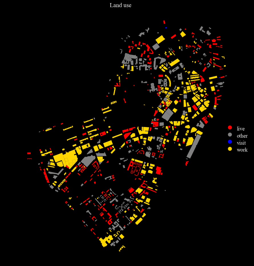
The land use can also be cagtegorised into 3 categories see https://journals.sagepub.com/doi/full/10.1177/0042098018819727

visit = ['adult_entertainment', 'attractions', 'culture', 'eating_drinking', 'sport', 'religious', 'social', 'sport']
work = ['agriculture', 'business_services', 'commercial', 'education_research', 'emergency_service', 'general_education',
        'industrial','medical_care', 'military_detainment','public', 'transport','utilities']
live = ['hospitality', 'residential']

categories = [visit, work, live]
strings = ['visit', 'work', 'live']
buildings = ci.classify_land_use(buildings, raw_land_use_column='land_use', new_land_use_column='DMA', categories=categories, strings=strings)

# visualising
from matplotlib.colors import LinearSegmentedColormap
colors = ['red', 'gray', 'blue', 'gold']
cmap = LinearSegmentedColormap.from_list('cmap', colors, N=len(colors))
fig = ci.plot_gdf(buildings, column = 'DMA', title = 'Land use', black_background = True, figsize = (10,10), cmap = cmap,
            legend = True)

Final scores

Defining Global indexes and components weights and assigning the score

global_indexes_weights = {'3dvis': 0.50, 'fac': 0.30, 'height': 0.20, 'area': 0.30, '2dvis':0.30, 'neigh': 0.20, 'road': 0.20}
global_components_weights = {'vScore': 0.40, 'sScore' : 0.30, 'cScore': 0.20, 'pScore': 0.10}
buildings = ci.compute_global_scores(buildings, global_indexes_weights, global_components_weights)

Define Local indexes and components weights

local_indexes_weights = {'3dvis': 0.50, 'fac': 0.30, 'height': 0.20, 'area': 0.40, '2dvis': 0.00, 'neigh': 0.30, 'road': 0.30}
local_components_weights = {'vScore': 0.25, 'sScore' : 0.35, 'cScore':0.10, 'pScore': 0.30}
rescaling_radius = 1000  # to define the local dimension, choose based on the extent of the case study area
buildings = ci.compute_local_scores(buildings, local_indexes_weights, local_components_weights, rescaling_radius =
                                    rescaling_radius)

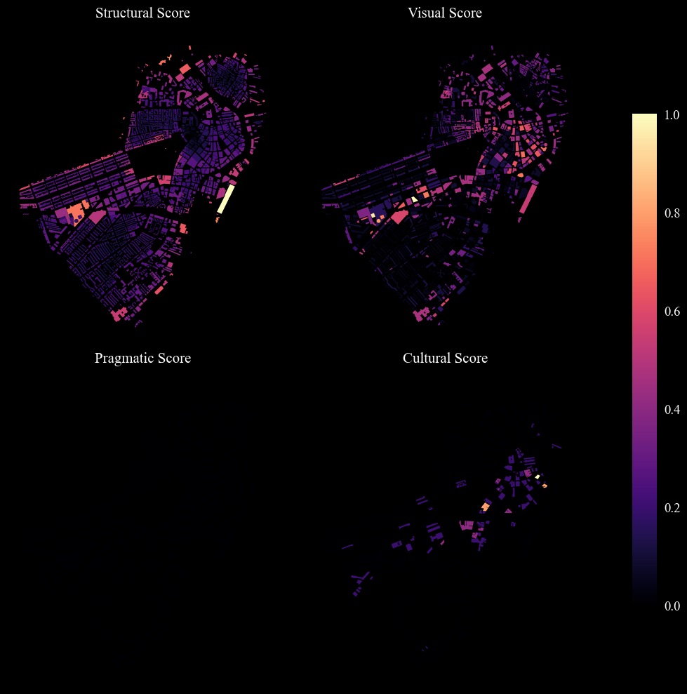
Visualisation of the Components

columns = ['sScore_sc', 'vScore_sc', 'pScore', 'cScore']
titles = ['Structural Score', 'Visual Score', 'Pragmatic Score', 'Cultural Score']
fig = ci.plot_grid_gdf_columns(gdf = buildings, columns = columns, titles = titles, black_background = True, figsize = (15,10),
                  scheme = 'fisher_jenks', cmap = 'magma', cbar = True, nrows = 2, ncols = 2)

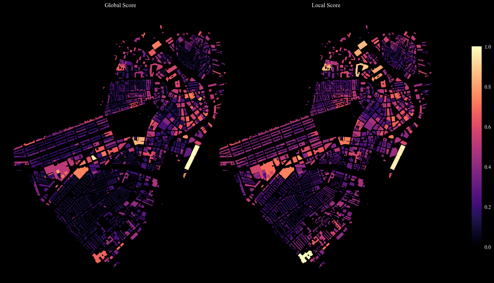
Visualisation of the Global and Local Landmark Scores

columns = ['gScore_sc', 'lScore_sc']
titles = ['Global Score', 'Local Score']
fig = ci.plot_grid_gdf_columns(gdf = buildings, columns = columns, titles = titles, black_background = True, figsize = (20,10),
                  scheme = 'fisher_jenks', cmap = 'magma', cbar = True, nrows = 1, ncols = 2)

Exporting. The results are written to disk as GeoPackage files with GeoPandas’ to_file, ready to be reused in later notebooks or in external GIS software.

sight_lines.to_file(output_path+'_sight_lines.gpkg', driver='GPKG')
buildings.to_file(output_path+'_landmarks.gpkg', driver='GPKG')