
Districts (Local Files)#
District should be derived using a car-based street network and for an area that is larger than the case study area (see below, e.g. for the city centre of London one should use Greater London)
Functions from the cityImage API used in this notebook#
This notebook derives districts (Lynch’s regions) from a locally loaded street network by partitioning it into communities and turning those partitions into region polygons.
clean_network — Clean and simplify the network: remove duplicate nodes/edges, pseudo-nodes, dead-ends and self-loops, and repair topology.
plot_gdf — Plot a single GeoDataFrame with cityImage styling.
dual_gdf — Build the dual-graph GeoDataFrames, where street segments become nodes (their centroids) and intersections become links.
dual_graph_fromGDF — Build the dual NetworkX graph used for angular (dual) analysis.
identify_regions — Identify districts/regions from a graph partition (community detection).
rand_cmap — Build a random categorical colormap (useful for districts/partitions).
plot_grid_gdf_columns — Plot several columns of one GeoDataFrame as a grid of maps.
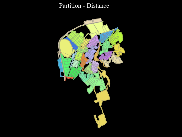
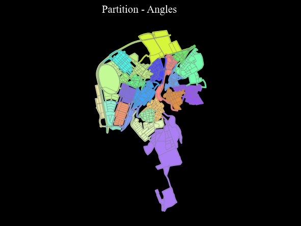
polygonise_partitions — Convert edge partitions into region polygons.
For the full list of functions and their parameters, see the API reference.
[2]:
import sys
from pathlib import Path

repo_root = Path.cwd().resolve().parents[1]
sys.path.insert(0, str(repo_root))

import cityImage as ci
import matplotlib.pyplot as plt
import matplotlib.font_manager as fm

fm.fontManager.addfont("times.ttf")
plt.rcParams["font.family"] = "Times New Roman"
[3]:
import osmnx as ox, networkx as nx, matplotlib.cm as cm, pandas as pd, numpy as np
import geopandas as gpd
from shapely.geometry import Point, mapping
%matplotlib inline

import warnings
warnings.simplefilter(action="ignore")
pd.options.display.float_format = '{:20.2f}'.format
pd.options.mode.chained_assignment = None

import cityImage as ci
Acquiring the Street Network#
[4]:
city_name = 'Tripoli'
epsg = 22780
crs = 'EPSG:'+str(epsg)
Loading the drive network from Local files#
[7]:
input_path = '../data/'+city_name+"/"+city_name

nodes_graph = gpd.read_file(input_path+'_nodes.gpkg', driver="GPKG")
edges_graph = gpd.read_file(input_path+'_edges.gpkg', driver="GPKG")

nodes_graph, edges_graph = nodes_graph.to_crs(crs), edges_graph.to_crs(crs)

nodes_graph.index, edges_graph.index, = nodes_graph.nodeID, edges_graph.edgeID
nodes_graph.index.name, edges_graph.index.name, = None, None
Cleaning and simplyfing the Street Network#
At the end of the previous section two files are obtained: nodes and edges (vertexes and links). Below, before creating the actual graph, the two datasets are cleaned, simplified and corrected.
Cleaning functions handle (through boolean parameters):
Duplicate geometries (nodes, edges).
Pseudo-nodes.
remove_islands: Disconnected islands.dead_endsDead-end street segments.self_loopsSelf-Loops.same_vertexes_edgesEdges with same from-to nodes, but different geometries.fix_topologyThis creates nodes and breaks street segments at intersections. It is primarily useful for poorly formed datasets (usually OSM deerived networks are topologically correct). It accounts for segments classified as bridges or tunnels in OSM.
same_vertexes_edges handles edges with same pair of u-v nodes but different geometries. When True, it derives a center line between the two segments, unless one of the two segments is longer than the other (>10%). In this case, the shorter segment is deleted.
[8]:
nodes_graph, edges_graph = ci.clean_network(nodes_graph, edges_graph, dead_ends = True, remove_islands = True,
                            same_vertexes_edges = True, self_loops = True, fix_topology = False)
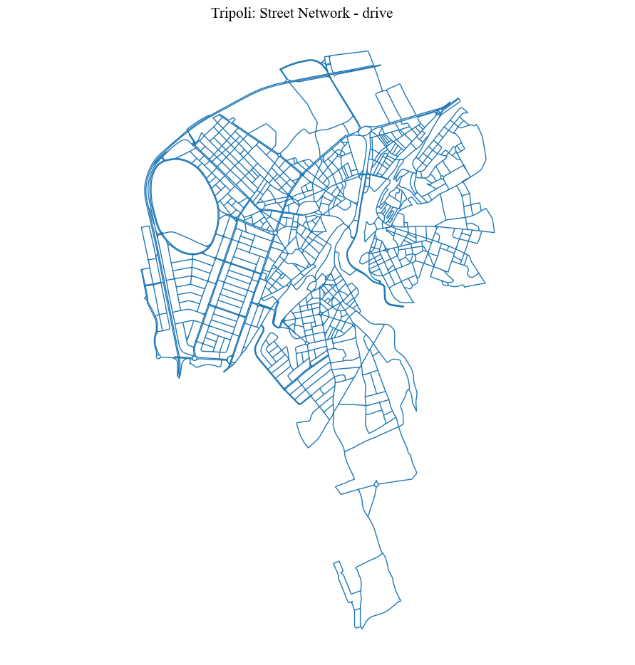
Visualisation. The cell below maps the result using the cityImage plotting helpers such as plot_gdf; see the Plotting section of the API reference for all styling options.
[9]:
fig = ci.plot_gdf(edges_graph, black_background = False, figsize = (10,10), title = city_name+': Street Network - drive')
District identification#
[10]:
# creating the dual_graph
nodesDual_graph, edgesDual_graph = ci.dual_gdf(nodes_graph, edges_graph, epsg)
dual_graph = ci.dual_graph_fromGDF(nodesDual_graph, edgesDual_graph)
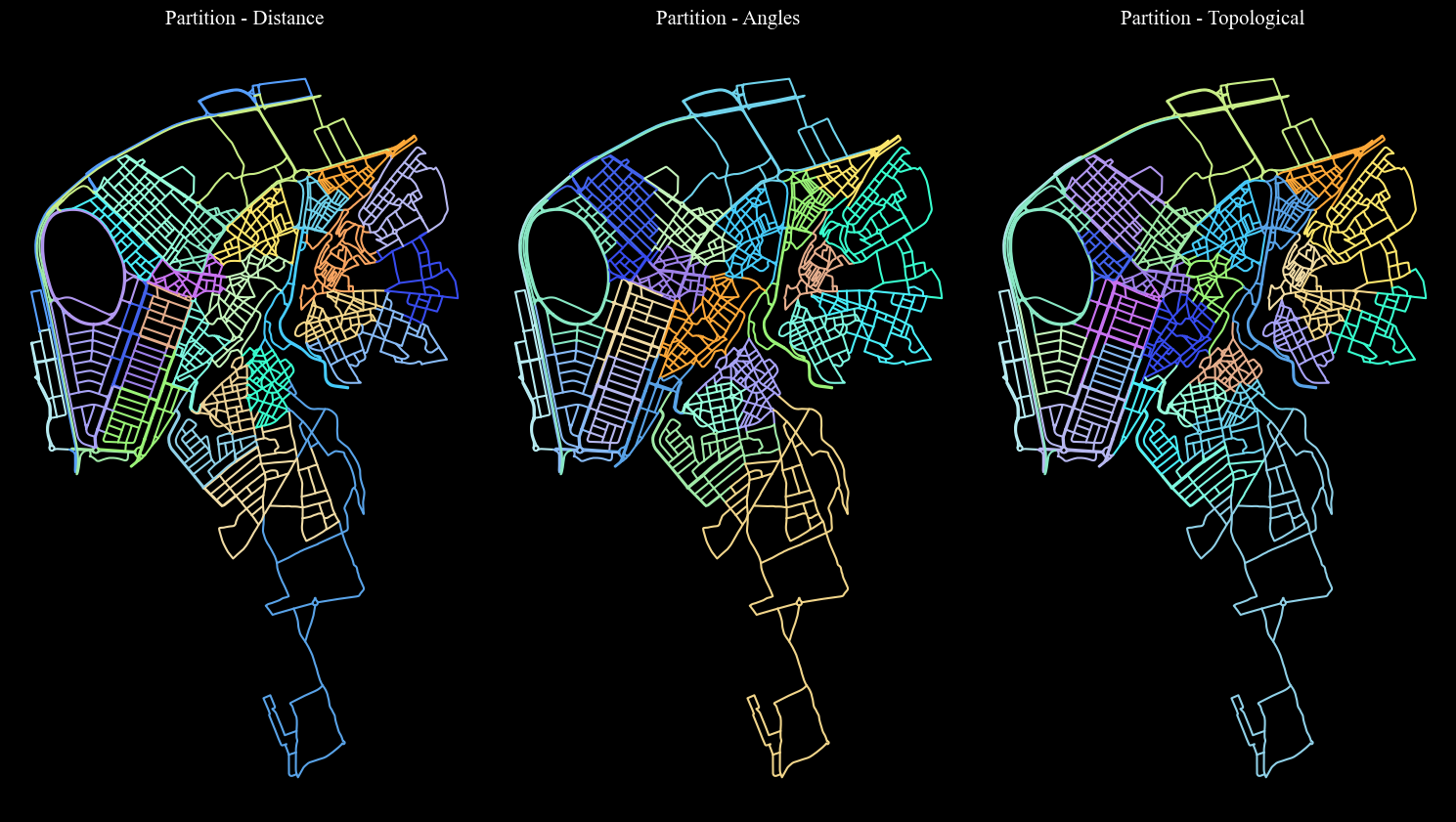
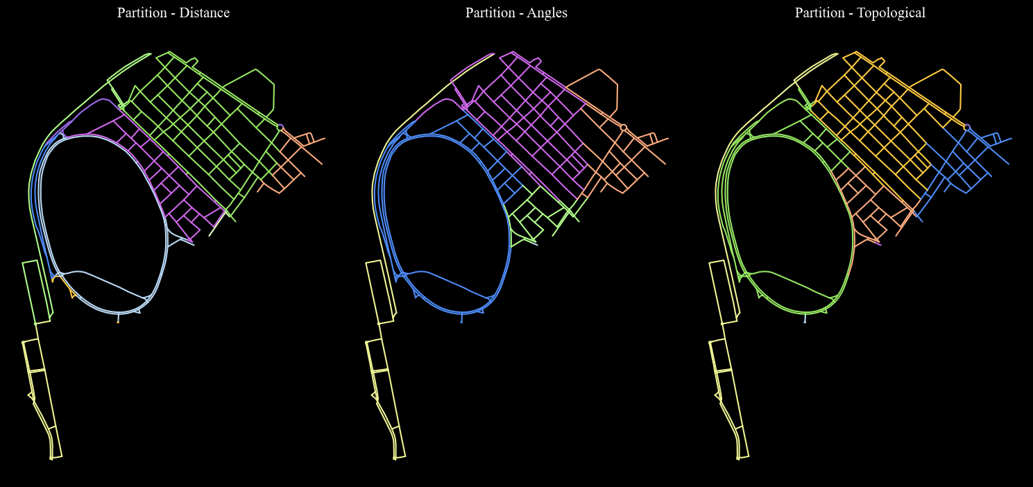
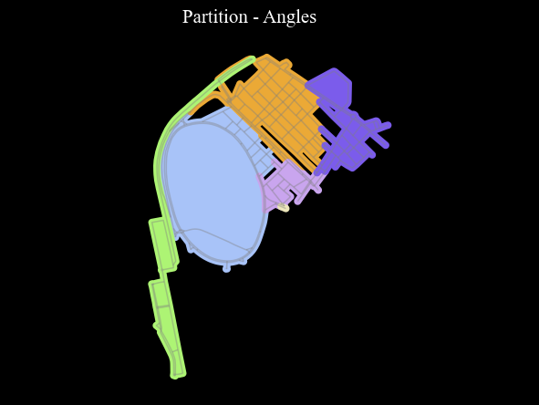
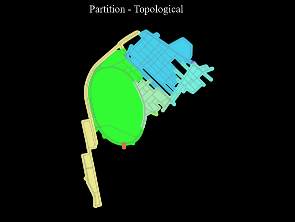
Different weights can be used to extract the partitions. None indicates that no weights will be used (only topological relationships will matter). The function returns a GeoDataFrame with partitions assigned to edges, with column named as p_name_weight (e.g. p_length).
[11]:
weights = ['length', 'rad', None]
districts = edges_graph.copy()
for weight in weights:
    districts = ci.identify_regions(dual_graph, districts, weight = weight)
Visualisation. The cell below maps the result using the cityImage plotting helpers such as plot_gdf; see the Plotting section of the API reference for all styling options.
[12]:
columns = ['p_length','p_rad', 'p_topo']
titles = ['Partition - Distance', 'Partition - Angles', 'Partition - Topological']

nlabels = max([len(districts[column].unique()) for column in columns])
cmap = ci.rand_cmap(nlabels = nlabels, type_color='bright')
fig = ci.plot_grid_gdf_columns(districts, columns = columns, titles = titles, geometry_size = 1.5, cmap = cmap, black_background = True,
                  legend = False, figsize = (15, 10), ncols = 3, nrows = 1)
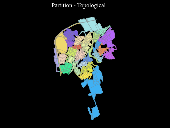
[13]:
for n, column in enumerate(columns):
    cmap = ci.rand_cmap(nlabels = len(districts[column].unique()), type_color='bright')
    partitions = ci.polygonise_partitions(districts, column, convex_hull = False)
    ci.plot_gdf(partitions, column = column, cmap = cmap, title =  titles[n], black_background = True,  figsize = (7, 5),
               base_map_gdf = districts, base_map_color = 'grey', base_map_zorder = 1)
Exporting. The results are written to disk as GeoPackage files with GeoPandas’ to_file, ready to be reused in later notebooks or in external GIS software.
[15]:
# provide path
from pathlib import Path

# provide path
output_dir = Path("../output")
output_dir.mkdir(parents=True, exist_ok=True)

output_file = output_dir / f"{city_name}_edges_districts.gpkg"
districts_export = districts.copy()
for col in districts_export.columns:
    if col != districts_export.geometry.name:
        districts_export[col] = districts_export[col].apply(
            lambda x: ", ".join(map(str, x)) if isinstance(x, (list, tuple, set)) else x
        )

districts_export.to_file(output_file, driver="GPKG")
Optional: Assigning regions to a sub-case study area’s network (From OSM relation or polygon)#
[19]:
# study_area_polygon = ox.geocode_to_gdf("Tripoli, Lebanon").to_crs(crs).iloc[0].geometry
study_area_polygon = gpd.read_file("../data/"+city_name+"/Tripoli_studyArea.gpkg",  driver="GPKG").iloc[0].geometry.buffer(50)
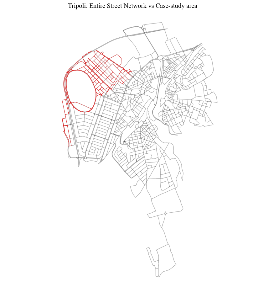
el_mina_tripoli_districts = districts[districts.geometry.within(study_area_polygon)]
Visualisation. The cell below maps the result using the cityImage plotting helpers such as plot_gdf; see the Plotting section of the API reference for all styling options.
[20]:
fig = ci.plot_gdf(el_mina_tripoli_districts, scheme = None,  black_background = False, figsize = (10,10), title =
              city_name+': Entire Street Network vs Case-study area', color = 'red', geometry_size = 0.5,
             base_map_gdf = districts, base_map_color = 'black', base_map_alpha = 0.3)
[21]:
columns = ['p_length','p_rad', 'p_topo']
titles = ['Partition - Distance', 'Partition - Angles', 'Partition - Topological']

nlabels = max([len(el_mina_tripoli_districts[column].unique()) for column in columns])
cmap = ci.rand_cmap(nlabels = nlabels, type_color='bright')
fig = ci.plot_grid_gdf_columns(el_mina_tripoli_districts, columns = columns, titles = titles, geometry_size = 1.5, cmap = cmap, black_background = True,
                  legend = False, figsize = (15, 10), ncols = 3, nrows = 1)
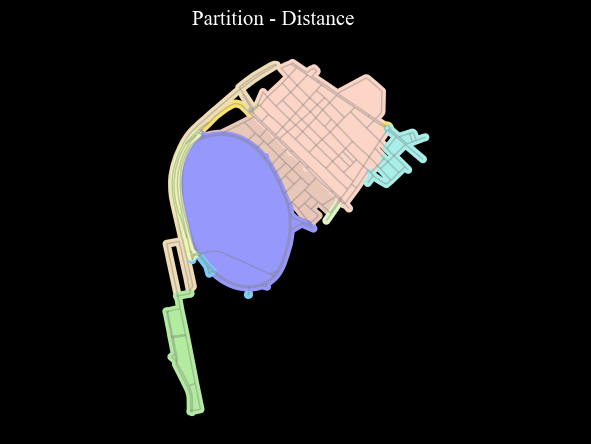
[22]:
for n, column in enumerate(columns):
    cmap = ci.rand_cmap(nlabels = len(el_mina_tripoli_districts[column].unique()), type_color='bright')
    partitions = ci.polygonise_partitions(el_mina_tripoli_districts, column, convex_hull = False)
    ci.plot_gdf(partitions, column = column, cmap = cmap, title =  titles[n], black_background = True,  figsize = (7, 5),
               base_map_gdf = el_mina_tripoli_districts, base_map_color = 'grey', base_map_zorder = 1)
Exporting. The results are written to disk as GeoPackage files with GeoPandas’ to_file, ready to be reused in later notebooks or in external GIS software.
[23]:
el_mina_tripoli_districts.to_file("../output/el_mina_tripoli_districts.gpkg", driver="GPKG")